How Vector Search Works: Chroma, pgvector and Qdrant
How embeddings work, why HNSW struggles with filters, and how Chroma, pgvector and Qdrant differ when searching by meaning.
- Section
- Technology
- Date
- Reading
- 30 minutes
- Source
- Qdrant Documentation
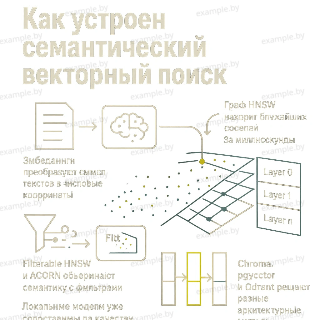
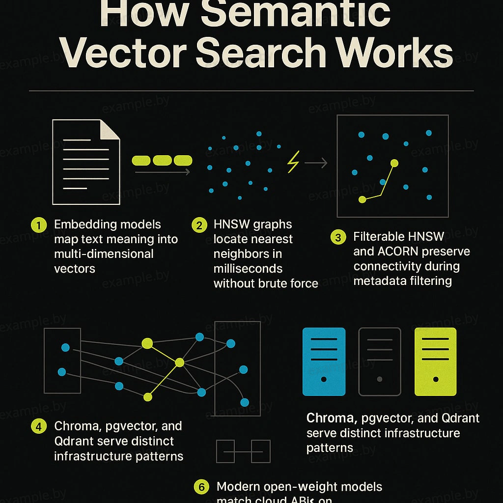
Imagine you have a million documents, user profiles or product descriptions.
A user types a query:
“Find specialists who have worked on AI products and launched their own startups.”
Yet none of the matching profiles may contain that exact wording.
One person wrote “Co-founder of an ML startup”. Another wrote “Built an LLM-powered SaaS from scratch”. A third described their experience as “Machine Learning Engineer, early-stage ventures”.
Traditional keyword search may miss some of these matches. Modern semantic search can link texts even when they use entirely different words.
How is that possible?
The technology rests on three components:
An embedding model converts information into mathematical vectors.
A vector database stores these representations and makes it possible to search for similar ones efficiently.
A search algorithm finds the nearest vectors without comparing every query against the entire database.
But the most interesting part begins when ordinary business conditions are added to semantic similarity: country, profession, document age, product category or user access rights.
This is where HNSW, Filterable HNSW, ACORN and other engineering solutions come in.
Let’s walk through the whole technology chain, from the mathematical foundations to production architecture.
1. What embeddings are and how a machine represents meaning with numbers
A computer does not understand words the way a human does. For search algorithms, text has to be represented as numbers.
An embedding is a numerical vector that a neural network model creates for an object: a text, an image, audio or another type of data.
For a text model, the process looks roughly like this:
          SOURCE TEXT
               │
               ▼
       ┌──────────────┐
       │ Tokenization │
       └──────────────┘
               │
               ▼
       ┌─────────────────┐
       │ Embedding Model │
       │   Transformer   │
       └─────────────────┘
               │
               ▼
        FEATURE VECTOR

    [ 0.12, -0.48, 0.91,
      0.07,  0.33, ... ]

               │
               ▼
         VECTOR SEARCH
For example, a model can convert the sentence:
“A software developer with experience building AI products”
into a vector of 1,024 numbers.
Another text:
“Software engineer building machine learning applications”
gets a vector of its own.
If the embedding model has been well trained for such tasks, these vectors can end up close to each other in a high-dimensional space.
Why does closeness of vectors mean closeness of meaning?
During training, the model learns to represent certain regularities of language through numerical parameters.
Texts with similar meanings often receive similar representations.
But one caveat is important: an embedding is not a perfect mathematical record of meaning.
A model can make mistakes, confuse context, handle negation poorly, or treat as similar documents that describe opposite actions.
For example:
- “The company is looking for investors.”
- “The company is not looking for investors.”
For some embedding models these sentences may turn out to be quite close, because most of their content is the same.
So semantic similarity is not the same as logical equivalence.
How is similarity measured?
One of the most popular methods is cosine similarity.
Mathematically:
Here:
- and are two vectors.
- is their dot product.
- and are the lengths of the vectors.
Cosine similarity measures how closely the directions of the vectors coincide.
For nonzero vectors, the value lies between −1 and 1.
The closer the value is to 1, the more similar the directions.
It is important that this is a mathematical measure of closeness, not the probability that two documents mean the same thing.
A value of 0.85 does not mean “85% match in meaning.”
2. How much memory do embeddings take?
Suppose each text is represented by a vector of 1,536 numbers.
If each number is stored in Float32 format, it takes 4 bytes.
That gives:
That is about 6 KB per vector.
For a million vectors you need roughly 6.14 GB just to store the numbers.
And that does not yet include metadata, search indexes or the database’s internal structures.
Chart 1. Size of a vector array by dimensionality
An important conclusion follows.
The dimensionality of embeddings directly affects the cost of storing and processing data.
However, higher dimensionality does not guarantee better search quality.
A small modern model with 1,024 dimensions can outperform an older model with 3,072 dimensions.
There are other ways to save memory too: Float16, vector quantization, and dimensionality reduction with models that support Matryoshka Representation Learning (MRL).
But each approach needs to be tested for its effect on search quality.
3. Why can’t we simply compare all the vectors?
Suppose we have built a system with 10 million documents.
A user sends a query. Its text is converted into an embedding, and then we need to find the 10 nearest vectors.
The naive algorithm looks like this:
              QUERY
                │
                ▼
       [0.12, 0.43, ...]
                │
                ▼
    ┌───────────────────────┐
    │ Compare with vector 1 │
    │ Compare with vector 2 │
    │ Compare with vector 3 │
    │          ...          │
    │ Compare to 10,000,000 │
    └───────────────────────┘
                │
                ▼
            SORTING
                │
                ▼
             TOP-10
This approach is called exact nearest neighbor search.
It has an important advantage: as long as distances are computed correctly, it finds the true nearest vectors.
But it has to compute the distance to every candidate.
If the database holds millions of objects and thousands of queries arrive at the same time, this approach becomes expensive.
To solve the problem, engineers use ANN, Approximate Nearest Neighbor Search.
Its idea is simple:
Instead of checking all objects, let’s try to quickly find the region of space where the best-matching results are most likely to be.
There are different approaches to ANN: graph indexes, clustering, quantization and combinations of them.
One of the most widespread graph algorithms is HNSW.
4. HNSW: how to search among millions of vectors without checking them all
HNSW stands for Hierarchical Navigable Small World.
It is an algorithm that organizes vectors into a multi-layer graph.
To grasp the idea, picture a city.
If we are looking for a particular house, we don’t need to check every house in the country.
We can use a hierarchy:
        COUNTRY
           │
           ▼
          CITY
           │
           ▼
        DISTRICT
           │
           ▼
         STREET
           │
           ▼
          HOUSE
HNSW follows similar logic, although its layers are not predefined geographic or semantic categories.
The algorithm builds links between vectors that let it move quickly through the space.
What an HNSW graph looks like
A simplified diagram:
LAYER 2, long-range jumps

        A ────────────── F
        │                │


LAYER 1, intermediate links

        A ───── C ────── F
        │       │        │
        B ───── D ────── G


LAYER 0, detailed graph

    A ─ B ─ C ─ D ─ E
    │   │   │   │   │
    F ─ G ─ H ─ I ─ J
    │   │   │   │   │
    K ─ L ─ M ─ N ─ O
The diagram is schematic: the real graph structure is irregular, and its links are determined by vector proximity and by the index-building procedure.
The upper layers contain relatively few nodes. They allow large jumps.
The bottom layer contains all the indexed vectors and much more detailed links.
The search starts at the top layer and gradually descends.
How does the algorithm choose a path?
Suppose the search is currently at node A.
The algorithm examines the available neighbors and looks for the direction that brings it closer to the query.
                       QUERY
                         ★
                         │
                D ────── E
               /         │
              C          F
             /           │
            B            G
           /
          A

      Starting point
In reality the search is not limited to a single chain: the algorithm maintains a set of candidates and explores several possible moves.
The key advantage is that it usually does not need to visit all the nodes.
Three important HNSW parameters
M determines the number of links between graph nodes.
A large M can improve search quality but increases memory consumption.
efConstruction controls the number of candidates considered while the graph is being built.
Raising it usually makes index construction more expensive but may improve the quality of the links.
efSearch controls the breadth of the search at query time.
The more candidates the algorithm considers, the higher the potential recall, but the more computation is required.
Here we meet a classic engineering trade-off:
Speed ↔ search quality ↔ memory consumption.
HNSW does not guarantee that it will always find the mathematically nearest neighbors. That is why its results are usually compared with exact search. (github.com, qdrant.tech)
5. Filterable HNSW: what happens when filters have to be taken into account?
In real applications, it is rarely enough to simply find the ten nearest vectors.
A query usually contains additional conditions.
For example:
Find the most similar specialists who live in Germany, have AI experience and are available for new projects.
This gives us:
SEMANTIC SEARCH

Similarity of professional experience
                │
                +
                │
STRUCTURED FILTERS
                │
                ├── country = Germany
                ├── availability = true
                └── experience >= 5 years
                │
                ▼
             TOP-10
And here a problem arises.
Why can plain HNSW work poorly with filters?
Imagine a database of a million users.
After all the conditions are applied, only 5,000 suitable candidates remain, or 0.5% of the database.
There are three main ways to organize the search.
The first approach: post-filtering.
First we find the 100 most similar vectors, then we discard the unsuitable ones.
If suitable users are distributed roughly uniformly, a hundred results will contain on average only 0.5 suitable users.
As a result, the search may return an empty list even though the database holds thousands of suitable candidates.
The second approach: pre-filtering.
First we select the 5,000 suitable users, then compute distances to all of their vectors.
This yields an exact result, provided distances are computed for all the selected objects.
However, with hundreds of thousands of suitable candidates, this approach can become expensive.
The third approach: filter-aware search.
What if the search algorithm itself took the constraints into account while moving through the graph?
This is exactly the problem that Filterable HNSW addresses.
How Filterable HNSW works in Qdrant
Ordinary HNSW builds links based on vector proximity.
But nodes that match a filter may be separated by nodes that don’t.
Consider:
           ORDINARY HNSW

      A (Germany, AI)
              │
              ▼
       B (France, AI)
              │
              ▼
      C (Germany, AI)


Filter: country = Germany
Nodes A and C pass the filter, but B does not.
If the algorithm restricts traversal to matching nodes, it risks losing the path from A to C.
Qdrant solves the problem with additional links.
          FILTERABLE HNSW

      A (Germany, AI)
        │           ╲
        │            ╲
        ▼             ╲
  B (France, AI)       ╲
        │               ╲
        ▼                ▼
      C (Germany, AI) ◄══╝


════ Extra link,
     useful for filtering
This is a schematic illustration: Qdrant does not connect every pair of objects with identical metadata.
Instead, while building the graph, the system adds links based on the indexed payload values.
In other words, the graph adapts not only to vector proximity but also to future search conditions.
For this, Qdrant uses two kinds of indexes:
- A vector index for finding similar vectors.
- A payload index for filtering on structured data.
Payload indexes also make it possible to estimate the number of matching objects and choose a query execution strategy.
That is why Qdrant can use either approximate graph search or exact brute-force search over a limited set of candidates.
One important detail: it is recommended to create payload indexes before loading data. If they are created after the HNSW graph has been built, obtaining the additional links requires rebuilding the graph index. (qdrant.tech)
And what is ACORN?
Filterable HNSW does not solve absolutely every problem.
Suppose the system filters simultaneously by country, profession, document age and several categories.
Qdrant adds extra links for individual indexed fields, but not for every possible combination of their values.
As a result, with several strict filters the graph can still lose useful paths.
For such situations Qdrant supports ACORN, starting with version 1.16.
The core idea of ACORN is to expand graph traversal.
If the nearest neighbor does not match the filter, the algorithm can explore that neighbor’s neighbors.
             QUERY
               │
               ▼
          A, matches
               │
               ▼
          B, excluded
               │
               ▼
          C, matches


    Ordinary restricted traversal
    can lose a useful path.

    ACORN explores the second hop,
    even when B fails the filter.
This can improve recall in complex scenarios, but it requires extra computation.
So ACORN is not a free speedup. It is a mechanism for improving search quality, especially with complex filters. (qdrant.tech, qdrant.tech)
6. Chroma, pgvector and Qdrant: three approaches to one problem
Now we understand what embeddings, vector search and HNSW are.
But a practical question arises: where should vectors be stored, and which technology should you choose?
Let’s look at three popular solutions.
Chroma: an AI-oriented database
Chroma is an open-source system focused on storing and searching data for AI applications.
Its core abstraction is the collection.
A collection contains items, each of which can have an identifier, a document, an embedding and metadata.
For example:
import chromadb

client = chromadb.PersistentClient(path="./data")

collection = client.get_or_create_collection(
    name="articles"
)

collection.add(
    ids=["article-1", "article-2"],
    documents=[
        "How vector search works",
        "Principles of building neural networks"
    ]
)

results = collection.query(
    query_texts=["How do I find similar documents?"],
    n_results=2
)
In an example like this, Chroma can use a configured embedding function to convert text into vectors automatically.
This is convenient: a developer doesn’t have to build separate infrastructure for every stage of search right away.
A typical scenario:
     PDF / Markdown / HTML
               │
               ▼
          Text Chunks
               │
               ▼
        Embedding Model
               │
               ▼
          CHROMA DB
               │
               ▼
        Semantic Search
               │
               ▼
              LLM
               │
               ▼
             ANSWER
It is important that modern Chroma is no longer limited to local experiments.
It supports a local embedded mode, a standalone server and distributed deployment. Dense and sparse search, hybrid retrieval, full-text search and metadata filtering are available.
The distributed architecture uses separate services, object storage and SSD caching. So it would be wrong to call Chroma purely a tool for small prototypes. (docs.trychroma.com, docs.trychroma.com)
When is Chroma especially interesting?
When you need to quickly build a RAG application, document search, a research prototype or an AI assistant.
Note that Python’s embedded mode and the JavaScript client are not the same thing: the regular JS client uses a Chroma server or a cloud database.
pgvector: vector search inside PostgreSQL
pgvector takes a different approach.
Instead of running a separate specialized database, you can add vector support directly to PostgreSQL.
CREATE EXTENSION vector;

CREATE TABLE documents (
    id BIGSERIAL PRIMARY KEY,
    title TEXT,
    category TEXT,
    embedding VECTOR(1536)
);
Now PostgreSQL can run vector queries:
SELECT id, title
FROM documents
WHERE category = 'technology'
ORDER BY embedding <=> $1::vector
LIMIT 10;
The <=> operator computes cosine distance.
For approximate search, you can create an HNSW index:
CREATE INDEX documents_embedding_idx
ON documents
USING hnsw (embedding vector_cosine_ops);
The main advantage of pgvector is its integration with the familiar features of PostgreSQL.
              APPLICATION
                   │
                   ▼
              PostgreSQL
                   │
         ┌─────────┼─────────┐
         │         │         │
         ▼         ▼         ▼
       Users    Payments   Documents
                             │
                             ▼
                         pgvector
                             │
                             ▼
                       Vector Search
You can combine vector proximity with SQL filters, JOINs, transactions and ordinary indexes.
This is especially convenient when AI search is an add-on feature of an existing application.
There is, however, an important nuance.
In pgvector, when an approximate HNSW index is used, filtering with an ordinary WHERE is applied after the index scan.
As a result, strict conditions can reduce the number of results found.
To improve the situation, iterative scans, partial HNSW indexes, partitioning and other optimizations are available.
For example:
SET hnsw.iterative_scan = strict_order;
This setting lets the index scan continue when too few rows are found after filtering, within the configured limits. (github.com)
One more technical detail: pgvector’s standard HNSW index for the vector type supports up to 2,000 dimensions. For higher dimensionalities you can use halfvec, with indexing of up to 4,000 dimensions, or other approaches.
This matters when using models that produce vectors of 3,072 dimensions and above. (github.com)
Qdrant: a specialized vector search engine
Qdrant is designed around the task of searching vector representations efficiently.
It is especially interesting for systems in which semantic search is one of the product’s key features.
Its main capabilities include HNSW, Filterable HNSW, payload indexes, dense and sparse vectors, named vectors, hybrid search and the combination of results from several search stages.
For example, a single object can have several semantic representations.
                PRODUCT
                   │
       ┌───────────┼───────────┐
       │           │           │
       ▼           ▼           ▼

   Description   Image       Reviews
     Vector      Vector       Vector

       │           │           │
       └───────────┼───────────┘
                   │
                   ▼
                 QDRANT
                   │
                   ▼
          Multi-stage Search
This opens up possibilities for sophisticated recommendation systems.
For example, an online store can search for products simultaneously by text description, visual similarity and customer reviews.
Qdrant lets you store several named vectors for one object and build search scenarios around different representations of the data.
But does this mean Qdrant is always faster than Chroma or pgvector?
No.
Real performance depends on the specific workload, the data structure, index size, filter selectivity, search parameters and available memory.
On a small database, PostgreSQL may well be faster because there are no network hops between separate services.
For a large specialized search system, Qdrant may be more convenient thanks to its mechanisms for indexing, filtering and managing vector data.
The main difference between the three
They can be described in a single sentence each:
Chroma provides convenient AI-oriented infrastructure for retrieval.
pgvector adds vector search to an existing relational database.
Qdrant offers specialized infrastructure for complex vector search and filtering.
None of them is a universal winner.
7. Can high-quality embeddings be created locally?
The next question is no less interesting.
Suppose we have chosen Qdrant or Chroma.
Where do we get the embeddings themselves?
Do we have to use the OpenAI API? Or can an ordinary computer handle the job?
The answer: high-quality embeddings can certainly be computed locally.
Moreover, there are open models that outperform commercial APIs on some tasks.
Let’s look at a few examples.
Qwen3-Embedding-0.6B
A compact model with 600 million parameters.
It supports more than 100 languages, a context of up to 32 thousand tokens and embeddings of up to 1,024 dimensions.
It can be run on an ordinary computer, including one without a discrete graphics card, although performance will depend on the hardware.
Qwen3-Embedding-4B
A larger model with 4 billion parameters.
The maximum embedding dimensionality is 2,560.
It requires more memory and computing resources but can deliver better search quality.
BGE-M3
A multilingual embedding model that supports several ways of representing information: dense, sparse and multi-vector.
This makes it interesting for hybrid search, where both semantic proximity and specific words need to be taken into account.
How can model quality be compared?
For this there is MTEB (Massive Text Embedding Benchmark).
It evaluates models on a variety of tasks, including retrieval, classification, clustering and semantic similarity.
Let’s look at the results of one comparison snapshot published by the Qwen authors.
Chart 2. Quality of embedding models on Multilingual MTEB
In this comparison, even Qwen3-Embedding-0.6B outperforms OpenAI text-embedding-3-large on the average score.
However, several caveats are in order.
First, these are the results of a specific set of tests, not a universal quality rating.
Second, the comparison was published by the authors of the Qwen family, so it is best supplemented with independent measurements.
Third, different tasks demand different properties from embeddings.
A model that is good at finding similar sentences will not necessarily be the best at searching for products by part number or matching specialists to strict professional requirements.
Even so, the results demonstrate an important fact: local open-source models can already compete with powerful cloud solutions. (huggingface.co)
8. So why do many people still use OpenAI Embeddings?
Because quality is only one criterion.
A cloud API spares developers from having to run and maintain a model themselves.
There is no need to deal with GPUs, quantization, inference servers, batch processing and the allocation of computing resources.
Besides, generating embeddings through an API can cost surprisingly little.
At the time this material was prepared, OpenAI listed the following standard prices:
text-embedding-3-small: $0.02 per million input tokens.text-embedding-3-large: $0.13 per million input tokens.
Source: OpenAI API. (developers.openai.com)
A cost example
Suppose you need to create embeddings for 10,000 documents.
Each document contains 500 tokens on average.
The total volume:
That comes to roughly:
$0.10 with text-embedding-3-small.
$0.65 with text-embedding-3-large.
And this is the cost of the initial generation of embeddings, not a monthly storage fee.
Of course, processing search queries and updating documents will also consume tokens.
But for many small projects, API costs are so low that running a local inference server brings no noticeable economic benefit.
When do local models become especially attractive?
When autonomy, control over data, independence from an external API, or processing large streams of information on hardware you already own are important.
For example:
           PRIVATE DOCUMENTS
                   │
                   ▼
          LOCAL EMBEDDING MODEL
                   │
                   ▼
           LOCAL VECTOR DB
                   │
                   ▼
              LOCAL SEARCH
With fully local processing, the source documents do not have to be sent to a third-party API.
This is useful for personal AI assistants, corporate documents and offline applications.
At the same time, running locally should not automatically degrade the quality of the embeddings.
If the same model weights, tokenizer, precision and processing parameters are used, the results of local and server-side inference should be practically identical.
Differences can arise from quantization, computational quirks and incorrect model configuration.
For some models it even matters whether a special instruction is used for the search query.
For example, the authors of Qwen3 recommend supplying instructions that describe the retrieval task, since this can improve results. (huggingface.co)
9. What a modern semantic search architecture looks like
Now let’s put all the components together.
Suppose we are building a search system for a database of technical articles.
Users can search for material in natural language.
The system must take category, language and publication date into account.
And the results must not merely be semantically close, but actually answer the question.
One possible architecture looks like this:
                 DATA PIPELINE
                      │
                      ▼
            ┌─────────────────┐
            │ Documents       │
            │ Articles        │
            │ Knowledge Base  │
            └─────────────────┘
                      │
                      ▼
               Text Chunking
                      │
                      ▼
              Embedding Model
                      │
                      ▼
              Vector Database
                      │
                      ▼
               Vector Index


═════════════════════════════════════════


                  USER QUERY
                      │
                      ▼
              Query Processing
                      │
           ┌──────────┴──────────┐
           │                     │
           ▼                     ▼
     Embedding Model       Keyword Search
           │                     │
           ▼                     ▼
      Dense Search          Sparse / BM25
           │                     │
           └──────────┬──────────┘
                      │
                      ▼
              Result Fusion
                      │
                      ▼
              Metadata Filters
                      │
                      ▼
              Candidate Set
                      │
                      ▼
                 Reranker
                      │
                      ▼
                  FINAL TOP-K
                      │
                      ▼
                LLM / USER
This is a logical diagram, not a mandatory order of operations. In a real system, metadata can be filtered directly during retrieval, including through Filterable HNSW.
Two important components appear here that we haven’t yet discussed in detail.
Hybrid search: why combine vector and ordinary search?
Semantic search is good at finding matches in meaning.
But sometimes an exact match of words matters more.
For example:
“PostgreSQL error 23505.”
Here the number 23505 is a specific error code.
An embedding model may find articles about PostgreSQL uniqueness constraints, but a literal search for the code can give a more reliable result.
That is why modern systems often combine:
Dense search, semantic search over embeddings.
Sparse search / BM25, search that takes into account specific terms and their importance.
The results are then merged.
One common method is Reciprocal Rank Fusion (RRF).
It combines several ranked lists, taking the documents’ positions into account.
This approach is useful when a user query contains both natural language and important keywords.
Reranking: why isn’t the nearest vector always the best answer?
Suppose the vector database has found 100 candidates.
All of them are semantically close to the query.
But some answer the question better than others.
For a more precise assessment, you can use a reranker.
The scheme:
           USER QUERY
                │
                ▼
          VECTOR SEARCH
                │
                ▼
         100 CANDIDATES
                │
                ▼
             RERANKER
                │
                ▼
           BEST 10 RESULTS
An embedding model usually converts the query and the documents into independent vectors.
A reranker can analyze the query together with the text of a specific document and output a relevance score for the pair.
This lets it take into account details that were not obvious from the initial vector similarity.
But there is a trade-off: reranking additional candidates increases query processing time.
That is why a common strategy is to quickly obtain a limited set of candidates and then apply a more expensive model to them.
10. How to evaluate the quality of vector search properly
One common mistake is to choose a vector database solely on speed.
For example, system A runs a query in 8 ms, while system B takes 20 ms.
Can we say that A is better?
No, not until we know how relevant the results are.
Several important metrics are used for evaluation.
Recall@K
It shows what share of the relevant results was found.
There are, however, two different ways to apply it.
ANN Recall@K compares approximate search with exact search over the same vectors.
It lets you measure how well the index works.
For example, exact search found the ten nearest vectors, and ANN returned eight of them.
Then Recall@10 relative to exact search is 80%.
But this figure says nothing about how well the vectors themselves reflect meaning.
Retrieval Recall@K compares the results found with relevant documents known in advance.
It helps evaluate the quality of the search system from the standpoint of the user’s task.
These are fundamentally different measurements.
NDCG@K
Normalized Discounted Cumulative Gain takes into account not only whether relevant documents are present but also their positions.
If the most useful document is in first place, that is better than if it appears only in tenth place.
That is why NDCG is especially interesting for recommendation systems and search interfaces.
Latency
Query execution time.
But a single average value is not enough.
It is worth looking at p50, p95 and p99.
For example, if most queries run fast but every twentieth takes several seconds, the user experience can deteriorate considerably.
Throughput
The number of queries the system can handle per unit of time.
It is especially important to measure it under real concurrent load.
Memory usage
You need to account not only for the size of the vectors themselves but also for the memory taken by indexes, metadata and cache.
The main idea of evaluation
The quality of a full-fledged search system depends on at least two independent components:
This is not a formula for numerical calculation but a way to show the dependency.
Even a perfect vector index will not fix poor embeddings.
And conversely, a superb embedding model does not guarantee good results if the search algorithm loses suitable candidates.
11. How to choose a technology stack
After all these comparisons, we can formulate a few practical principles.
If you are building RAG or an AI assistant
Chroma can be a good starting option.
Especially if you need to quickly set up document search and experiment with models.
But as the project grows, it is worth separately checking the requirements for scaling, language support, filtering and infrastructure.
If your application already uses PostgreSQL
Start with pgvector.
It lets you add vector search without introducing a separate database.
For moderate data volumes and relatively simple search scenarios, this may be the most rational solution.
If vector search is a key feature of your product
Take a close look at Qdrant.
Especially if you need search across several representations of one object, complex filtering, hybrid retrieval and scalable specialized infrastructure.
If you need fully local AI features
You can use an open embedding model and a local vector database.
But keep in mind that the size of the model, the memory it takes and the speed of embedding generation will depend directly on the available hardware.
If you need the simplest possible operation
A cloud embedding API combined with an existing database often turns out to be economically attractive.
Especially in the early stages of a product.
12. Five common misconceptions about vector search
“The higher the dimensionality of the embeddings, the better the search.”
Not necessarily. Quality depends on the model’s architecture and training, not only on the number of values in the output vector.
“HNSW always returns the nearest objects.”
No. It is an approximate search algorithm. Its advantage is a good trade-off between speed and recall.
“A vector database understands the meaning of text by itself.”
Usually the semantic representation is created by an embedding model. The database is responsible for storing, indexing, filtering and searching these representations. Some systems can additionally integrate embedding generation.
“Plain cosine similarity is enough for complex search.”
Not always. With strict business conditions, exact terms and ranking requirements, you may need payload filters, hybrid search and reranking.
“Cloud embeddings are inherently better than local ones.”
This is no longer a universal rule. Quality depends on the specific model and task, and modern open-source solutions show competitive results.
There is one more architectural trap: you cannot simply swap the embedding model and keep searching over the old vectors, even if the dimensionality matches.
Different models create different vector spaces. When migrating, you must recompute the stored embeddings or maintain separate representations of the data for different models.
Conclusion. Search by meaning is not one technology but a whole system
Behind a simple user query lie several separate engineering problems.
Text has to be converted into a numerical representation.
Millions of vectors have to be stored efficiently.
Nearest neighbors have to be found without scanning the whole database.
Structured filters have to be taken into account.
Semantic and lexical search have to be combined.
And finally, you have to evaluate not only the speed of the response but also the quality of the results found.
Put it all together and you get the following architecture:
                 AI SEARCH SYSTEM

                       │
                       ▼
              EMBEDDING MODEL
             ┌─────────┴─────────┐
             │                   │
             ▼                   ▼
       OpenAI API            Local Model
                             Qwen / BGE
             │                   │
             └─────────┬─────────┘
                       │
                       ▼
                 VECTOR SPACE
                       │
                       ▼
                VECTOR DATABASE
             ┌─────────┼─────────┐
             │         │         │
             ▼         ▼         ▼
           Chroma   pgvector   Qdrant
             │         │         │
             └─────────┼─────────┘
                       │
                       ▼
                  ANN SEARCH
                    HNSW
                       │
                       ▼
                FILTERED SEARCH
                       │
                       ▼
                 HYBRID SEARCH
                       │
                       ▼
                    RERANKER
                       │
                       ▼
               RELEVANT RESULTS
Chroma, pgvector and Qdrant are not three generations of one technology, nor three options with inherently different levels of quality.
They are different architectural approaches to building search systems.
HNSW solves the problem of efficient search in a high-dimensional space. Filterable HNSW and ACORN help combine vector proximity with structured constraints. And modern embedding models, including local open-source ones, determine how well the information itself is represented in that space.
It is the interaction of these components that determines the final quality of AI search.
Perhaps the most interesting takeaway is that the development of vector search is gradually shifting developers’ attention from the question “how do we quickly find the nearest numbers?” to a much harder one:
How do we build a system that finds not merely mathematically similar objects, but genuinely useful information?
And the answer increasingly lies not in choosing one perfect database, but in a skillful combination of models, indexes, filters and ranking algorithms.
Key technical sources
For further reading and to verify the details:
- Chroma Documentation, Chroma’s architecture, collections, local and distributed modes.
- pgvector GitHub, the HNSW implementation, SQL queries, indexes and limitations.
- Qdrant: Indexing, payload indexes and Filterable HNSW.
- Qdrant: Search, search parameters and ACORN.
- Qwen3-Embedding, model descriptions, MTEB results and inference examples.
- MTEB Leaderboard, a comparison of embedding models.
- OpenAI Embeddings, models, the API and working with vector representations.
This material was prepared using the documentation available as of October [check: current year]. The MTEB figures cited come from a comparison snapshot published in 2025. The vector-size chart is based on a mathematical calculation; the architecture and algorithm diagrams are simplified for clarity.
Liked it? Save it for later.
 Technology · 16.10.26
The Life Cycle of a Star: From Nebula to Black Hole
 Technology · 13.10.26
How Smart Scales Track Muscle and Water
 Technology · 13.10.26
How to Gain Reach on UGC Platforms
 Technology · 07.10.26
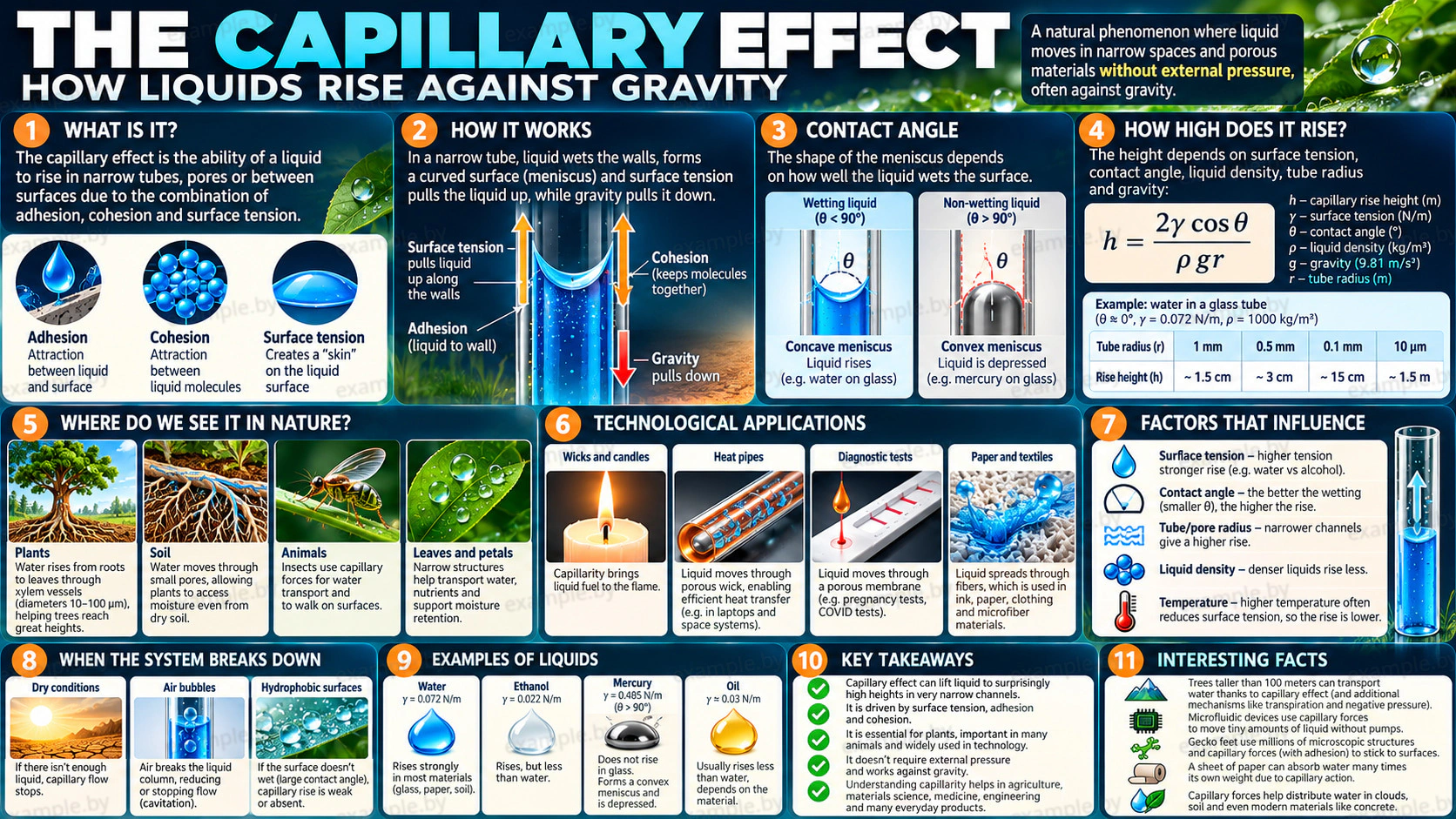
Capillary Action: Why Water Climbs Upward
 Technology · 04.10.26
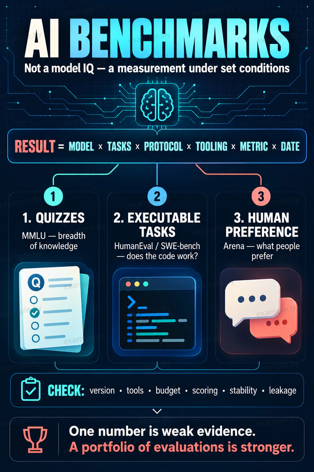
AI Benchmarks: Testing Models and Why Leaderboards Lie
 Medicine · 05.10.26
How Helicobacter pylori Survives Stomach Acid
 Medicine · 03.10.26
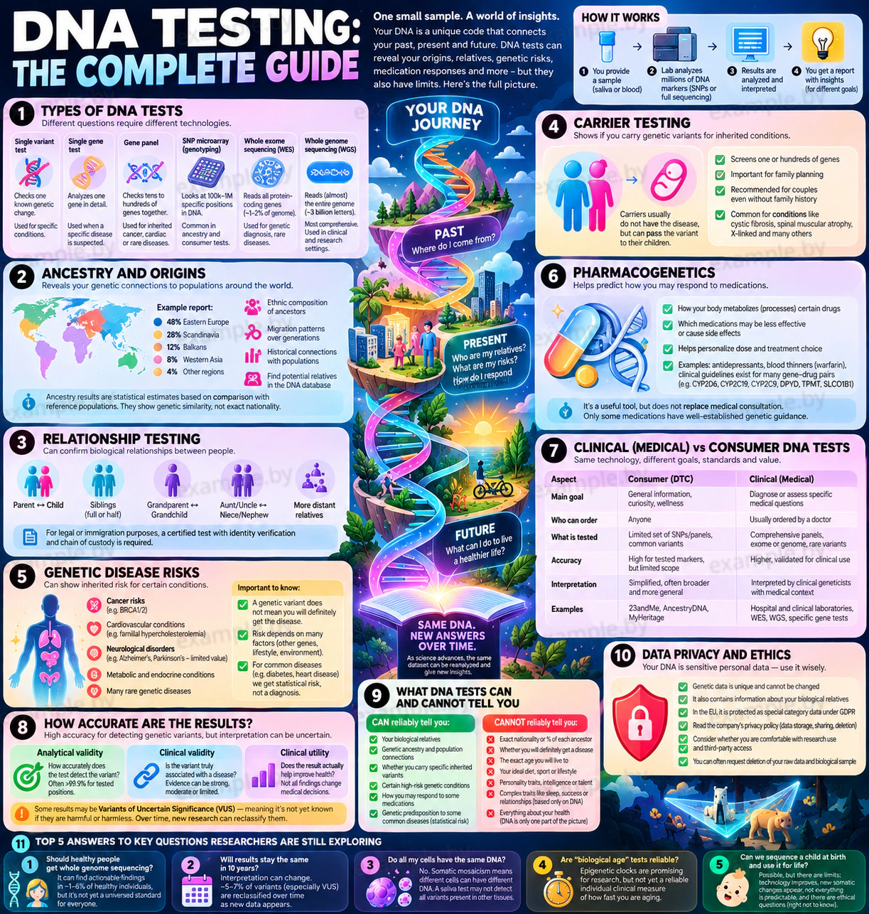
What DNA Tests Can Actually Reveal
 Culture · 27.10.26
Why One Family Can Have Different Surnames
 Biology · 19.10.26
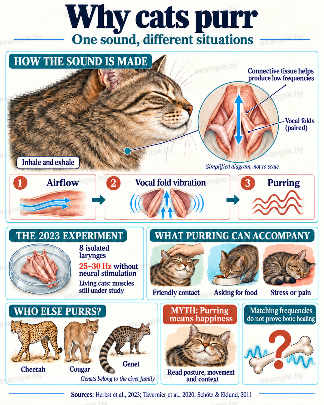
Why Cats Purr and What the Sound Really Means
 Culture · 18.10.26
How PR Works: Mechanisms, Limits and Trust
 Society · 18.10.26
Cypriot Pound or Lira: A Currency with Two Names
 Body · 18.10.26
The Art of the Pause: How to Speak Calmly and Confidently